FEMM Solver Test
介绍
本文档用于在Baffalo环境下,对FEMM求解器的验证。FEMM是开源的2D有限元方法的电磁仿真软件,其提供了友好的Matlab接口。
FEMM非常容易上手,其主要问题在于2D几何绘制非常不方便,导致其处理实际问题非常吃力,结合Bafflo的几何模块Point2D、Line2D和Surface2D可以更加方便的绘制几何,从而能在一定程度上弥补FEMM的不足。
以下案例一部分参考网上简单案例,还有一部分贴出了官方案例以供参考。
案例
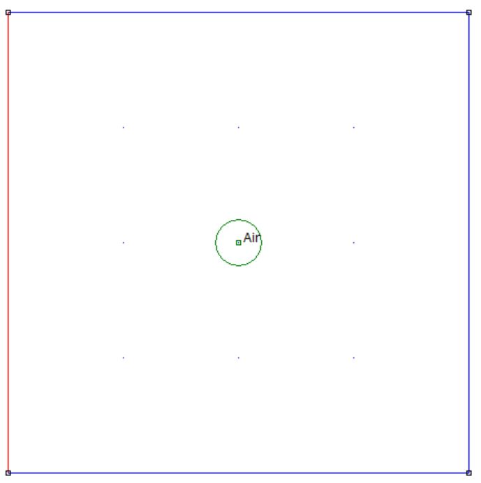
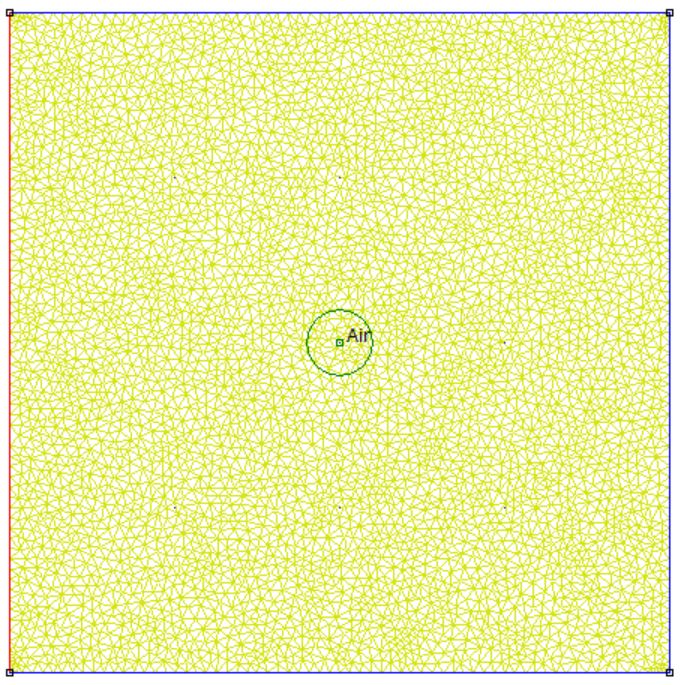
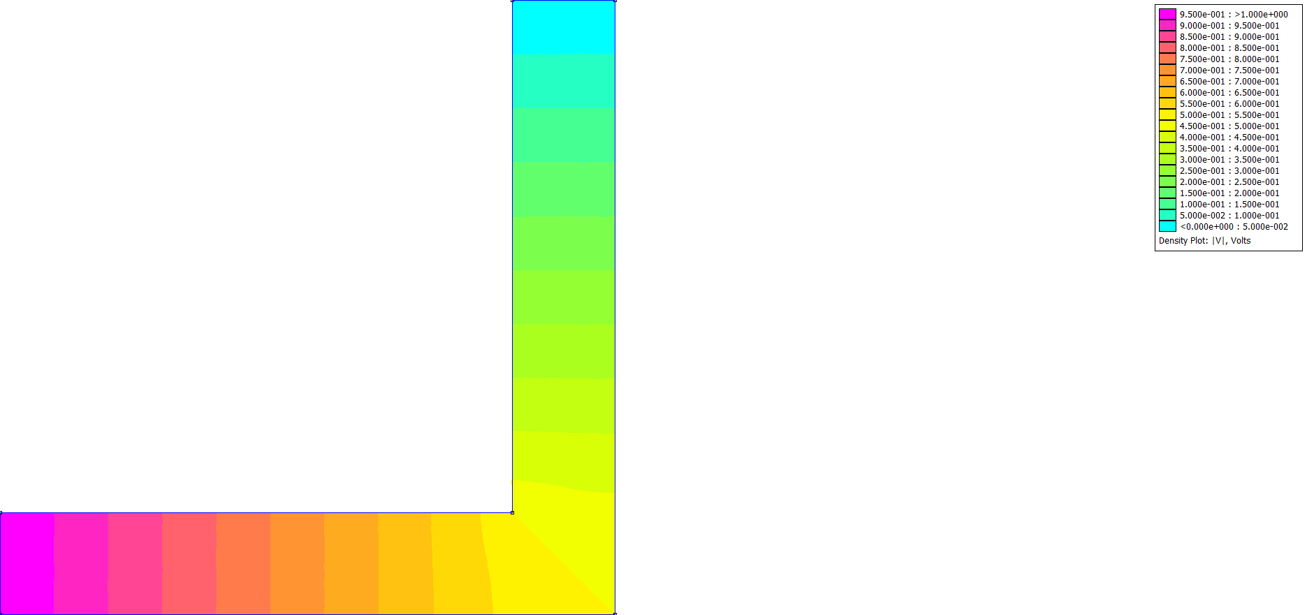
The box problem (Flag=1)
a=Point2D('Temp');
a=AddPoint(a,[0;1;1;0],[0;0;1;1]);
b=Line2D('Temp');
b=AddCurve(b,a,1);
S=Surface2D(b);
openfemm;
newdocument(1)
ei_probdef('millimeters','planar',1e-8,1,30)
FEMM_TransferSurface2D(S,'Type',1)
ei_addblocklabel(0.5,0.5);
ei_getmaterial('Air');
ei_selectlabel(0.5,0.5);
ei_setblockprop('Air',0,0.1,0);
ei_addboundprop('V=0',0,0,0,0,0);
ei_addboundprop('V=1',1,0,0,0,0);
ei_selectsegment(0.5,0);
ei_setsegmentprop('V=0',0.1,1,0,0,'<None>');
ei_clearselected
ei_selectsegment(1,0.5);
ei_setsegmentprop('V=0',0.1,1,0,0,'<None>');
ei_clearselected
ei_selectsegment(0.5,1);
ei_setsegmentprop('V=0',0.1,1,0,0,'<None>');
ei_clearselected
ei_selectsegment(0,0.5);
ei_setsegmentprop('V=1',0.1,1,0,0,'<None>');
ei_saveas('Box_problem.FEE')
ei_createmesh;
ei_analyze(0)
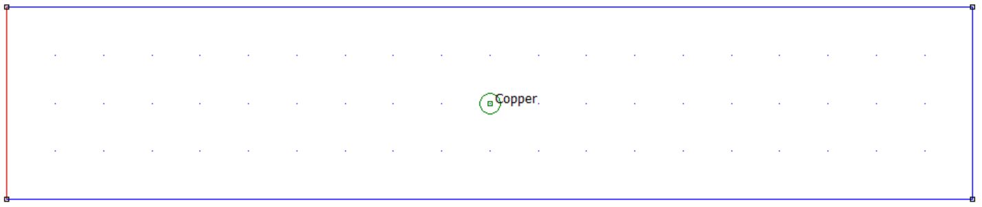
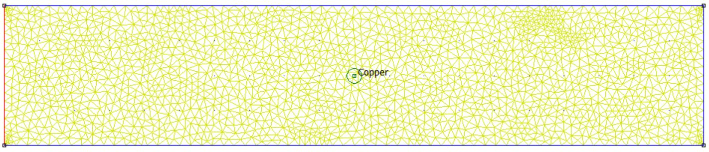
DC Conduction (Flag=2)
a=Point2D('Temp');
a=AddPoint(a,[0;5;5;0],[0;0;1;1]);
b=Line2D('Temp');
b=AddCurve(b,a,1);
S=Surface2D(b);
openfemm;
newdocument(3)
ci_probdef('millimeters','planar',0,1e-8,1,30)
FEMM_TransferSurface2D(S,'Type',3)
ci_addblocklabel(2.5,0.5);
ci_getmaterial('Copper');
ci_selectlabel(2.5,0.5);
ci_setblockprop('Copper',0,0.1,0);
ci_addboundprop('V=0',0,0,0,0,0);
ci_addboundprop('V=1',1,0,0,0,0);
ci_addboundprop('Insulation',0,0,0,0,2);
ci_selectsegment(2.5,0);
ci_setsegmentprop('Insulation',0.1,1,0,0,'<None>');
ci_clearselected
ci_selectsegment(5,0.5);
ci_setsegmentprop('V=0',0.1,1,0,0,'<None>');
ci_clearselected
ci_selectsegment(2.5,1);
ci_setsegmentprop('Insulation',0.1,1,0,0,'<None>');
ci_clearselected
ci_selectsegment(0,0.5);
ci_setsegmentprop('V=1',0.1,1,0,0,'<None>');
ci_saveas('DC_Conduction.FEC')
ci_createmesh;
ci_analyze(0)
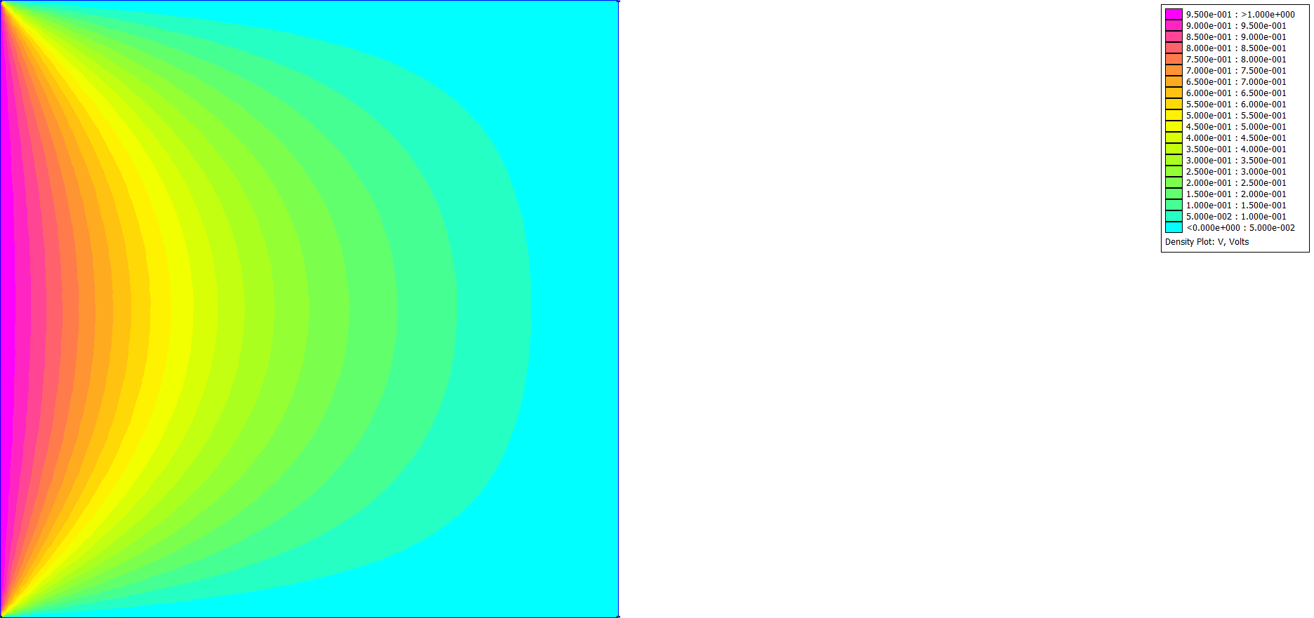
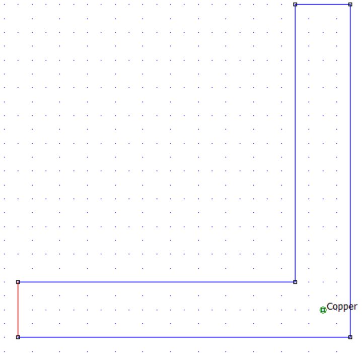
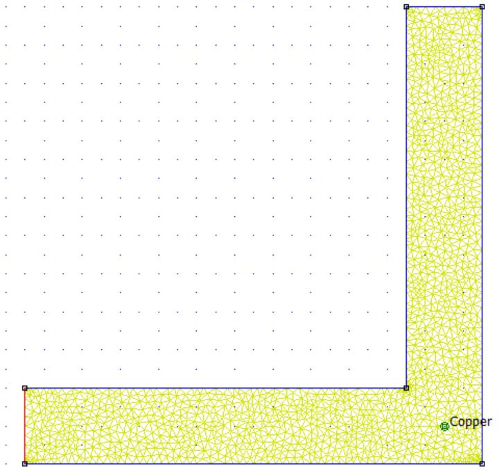
DC Condition L shape (Flag=3)
a=Point2D('Temp');
a=AddPoint(a,[0;6;6;5;5;0;0],[0;0;6;6;1;1;0]);
b=Line2D('Temp');
b=AddCurve(b,a,1);
S=Surface2D(b);
openfemm;
newdocument(3)
ci_probdef('centimeters','planar',0,1e-8,1,30)
FEMM_TransferSurface2D(S,'Type',3)
ci_addblocklabel(5.5,0.5);
ci_getmaterial('Copper');
ci_selectlabel(5.5,0.5);
ci_setblockprop('Copper',0,0.1,0);
ci_addboundprop('V=0',0,0,0,0,0);
ci_addboundprop('V=1',1,0,0,0,0);
ci_addboundprop('Insulation',0,0,0,0,2);
ci_selectsegment(3,0);
ci_setsegmentprop('Insulation',0.1,1,0,0,'<None>');
ci_clearselected
ci_selectsegment(6,3);
ci_setsegmentprop('Insulation',0.1,1,0,0,'<None>');
ci_clearselected
ci_selectsegment(5.5,6);
ci_setsegmentprop('V=0',0.1,1,0,0,'<None>');
ci_clearselected
ci_selectsegment(5,3.5);
ci_setsegmentprop('Insulation',0.1,1,0,0,'<None>');
ci_clearselected
ci_selectsegment(2.5,1);
ci_setsegmentprop('Insulation',0.1,1,0,0,'<None>');
ci_clearselected
ci_selectsegment(0,0.5);
ci_setsegmentprop('V=1',0.1,1,0,0,'<None>');
ci_saveas('DC_Conduction_Lshape.FEC')
ci_createmesh;
ci_analyze(0)
 |  |
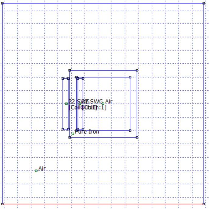
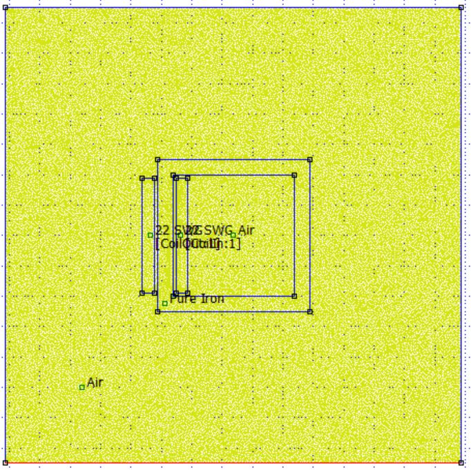
CloseCore (Flag=4)
a=Point2D('Temp');
a=AddPoint(a,[0;10;10;0],[0;0;10;10]);
a=AddPoint(a,[1;9;9;1],[1;1;9;9]);
a=AddPoint(a,[1.2;2;2;1.2],[1.2;1.2;8.8;8.8]);
a=AddPoint(a,[-1;-0.2;-0.2;-1],[1.2;1.2;8.8;8.8]);
a=AddPoint(a,[-10;20;20;-10],[-10;-10;20;20]);
b=Line2D('Temp');
b=AddCurve(b,a,1);
b1=Line2D('Temp');
b1=AddCurve(b1,a,2);
b2=Line2D('Temp');
b2=AddCurve(b2,a,3);
b3=Line2D('Temp');
b3=AddCurve(b3,a,4);
b4=Line2D('Temp');
b4=AddCurve(b4,a,5);
S=Surface2D(b);
S=AddHole(S,b1);
S1=Surface2D(b2);
S2=Surface2D(b3);
S3=Surface2D(b4);
openfemm;
newdocument(0)
mi_probdef(0,'centimeters','planar',1e-8,1,30)
FEMM_TransferSurface2D(S,'Type',0)
FEMM_TransferSurface2D(S1,'Type',0)
FEMM_TransferSurface2D(S2,'Type',0)
FEMM_TransferSurface2D(S3,'Type',0)
mi_addblocklabel(0.5,0.5);
mi_addblocklabel(1.5,5);
mi_addblocklabel(-0.5,5);
mi_addblocklabel(5,5);
mi_addblocklabel(-5,-5);
mi_addmaterial('Pure Iron',4000,4000,0,0,10.44,0,0,1,0,0,0,0,0)
mi_getmaterial('22 SWG');
mi_getmaterial('Air');
mi_addboundprop('A=0',0,0,0,0,0,0,0,0,0,0,0);
mi_addcircprop('CoilIn',-100,1);
mi_addcircprop('CoilOut',100,1);

mi_selectlabel(0.5,0.5);
mi_setblockprop('Pure Iron',0,0.2,'<None>',0,0,1);
mi_clearselected
mi_selectlabel(1.5,5);
mi_setblockprop('22 SWG',0,0.2,'CoilIn',0,0,1);
mi_clearselected
mi_selectlabel(-0.5,5);
mi_setblockprop('22 SWG',0,0.2,'CoilOut',0,0,1);
mi_clearselected
mi_selectlabel(5,5);
mi_setblockprop('Air',0,0.2,'<None>',0,0,1);
mi_clearselected
mi_selectlabel(-5,-5);
mi_setblockprop('Air',0,0.2,'<None>',0,0,1);
mi_clearselected

mi_selectsegment(20,5);
mi_setsegmentprop('A=0',0.2,1,0,0);
mi_clearselected
mi_selectsegment(5,20);
mi_setsegmentprop('A=0',0.2,1,0,0);
mi_clearselected
mi_selectsegment(-10,5);
mi_setsegmentprop('A=0',0.2,1,0,0);
mi_clearselected
mi_selectsegment(5,-10);
mi_setsegmentprop('A=0',0.2,1,0,0);
mi_saveas('CloseCore.FEM')
mi_createmesh;
mi_analyze(0)
 |  |
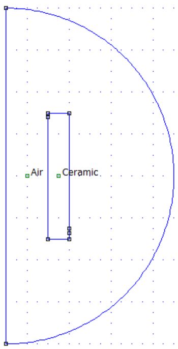
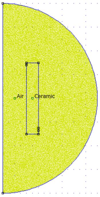
ACElec2 example (Flag=5)
openfemm;
create(3);
% define some parameters. These can then
% be used to draw the geometry parametrically
ri=1;
ro=1.5;
z=1.5;
% draw geometry of interest
ci_drawline(ri,-z,ri,z);
ci_drawline(ri,z,ro,z);
ci_drawline(ro,z,ro,-z);
ci_drawline(ri,-z,ro,-z);
ci_addnode(ri,z-0.1);
ci_addnode(ro,-z+0.15);
ci_addnode(ro,-z+0.25);
% draw boundary
ci_drawarc(0,-4,0,4,180,2);
ci_drawline(0,-4,0,4);
% add material definitions
ci_addmaterial('Air',0,0,1,1,0,0);
ci_addmaterial('Ceramic',1e-8,1e-8,6,6,0,0);
% add some block labels
ci_addblocklabel((ri+ro)/2,0);
ci_selectlabel((ri+ro)/2,0);
ci_setblockprop('Ceramic',0,0.05,0)
ci_clearselected;
ci_addblocklabel(ri/2,0);
ci_selectlabel(ri/2,0);
ci_setblockprop('Air',0,0.05,0)
ci_clearselected;
% Add some boundary properties
ci_addboundprop('U+', 5,0,0,0,0)
ci_addboundprop('U-',-5,0,0,0,0)
ci_selectsegment(ro,-z+0.1);
ci_selectsegment((ro+ri)/2,-z);
ci_selectsegment(ri,0);
ci_setsegmentprop('U+',0,1,0,0,'<None>');
ci_clearselected;
ci_selectsegment((ro+ri)/2,z);
ci_selectsegment(ro,0);
ci_setsegmentprop('U-',0,1,0,0,'<None>');
ci_clearselected;
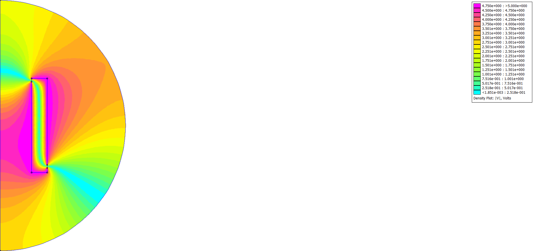
ci_zoomnatural;
% Save, analyze, and view results
ci_saveas('ACElec2.fec');
ci_analyze;
ci_loadsolution;
 |  |
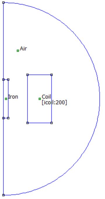
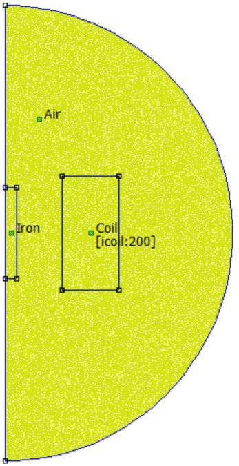
Coil (Flag=6)
disp('Wound Copper Coil with an Iron Core');
disp('David Meeker')
disp('dmeeker@ieee.org')
disp(' ');
disp('This program consider an axisymmetric magnetostatic problem');
disp('of a cylindrical coil with an axial length of 100 mm, an');
disp('inner radius of 50 mm, and an outer radius of 100 mm. The');
disp('coil has 200 turns and the coil current is 20 Amps. There is');
disp('an iron bar 80 mm long with a radius of 10 mm centered co-');
disp('axially with the coil. The objective of the analysis is to');
disp('determine the flux density at the center of the iron bar,');
disp('and to plot the field along the r=0 axis. This analysis');
disp('defines a nonlinear B-H curve for the iron and employs an');
disp('asymptotic boundary condition to approximate an "open"');
disp('boundary condition on the edge of the solution domain.');
disp(' ');
% The package must be initialized with the openfemm command.
% This command starts up a FEMM process and connects to it
openfemm;
% We need to create a new Magnetostatics document to work on.
newdocument(0);
% Define the problem type. Magnetostatic; Units of mm; Axisymmetric;
% Precision of 10^(-8) for the linear solver; a placeholder of 0 for
% the depth dimension, and an angle constraint of 30 degrees
mi_probdef(0, 'millimeters', 'axi', 1.e-8, 0, 30);
% Draw a rectangle for the steel bar on the axis;
mi_drawrectangle([0 -40; 10 40]);
% Draw a rectangle for the coil;
mi_drawrectangle([50 -50; 100 50]);
% Draw a half-circle to use as the outer boundary for the problem
mi_drawarc([0 -200; 0 200], 180, 2.5);
mi_addsegment([0 -200; 0 200]);
% Add block labels, one to each the steel, coil, and air regions.
mi_addblocklabel(5,0);
mi_addblocklabel(75,0);
mi_addblocklabel(30,100);
% Define an "asymptotic boundary condition" property. This will mimic
% an "open" solution domain
muo = pi*4.e-7;
mi_addboundprop('Asymptotic', 0, 0, 0, 0, 0, 0, 1/(muo*0.2), 0, 2);
% Apply the "Asymptotic" boundary condition to the arc defining the
% boundary of the solution region
mi_selectarcsegment(200,0);
mi_setarcsegmentprop(2.5, 'Asymptotic', 0, 0);
% Add some materials properties
mi_addmaterial('Air', 1, 1, 0, 0, 0, 0, 0, 1, 0, 0, 0);
mi_addmaterial('Coil', 1, 1, 0, 0, 58*0.65, 0, 0, 1, 0, 0, 0);
mi_addmaterial('LinearIron', 2100, 2100, 0, 0, 0, 0, 0, 1, 0, 0, 0);
% A more interesting material to add is the iron with a nonlinear
% BH curve. First, we create a material in the same way as if we
% were creating a linear material, except the values used for
% permeability are merely placeholders.
mi_addmaterial('Iron', 2100, 2100, 0, 0, 0, 0, 0, 1, 0, 0, 0);
% A set of points defining the BH curve is then specified.
bhcurve = [ 0.,0.3,0.8,1.12,1.32,1.46,1.54,1.62,1.74,1.87,1.99,2.046,2.08;
0, 40, 80, 160, 318, 796, 1590, 3380, 7960, 15900, 31800, 55100, 79600]';
% plot(bhcurve(:,2),bhcurve(:,1))
% Another command associates this BH curve with the Iron material:
mi_addbhpoints('Iron', bhcurve);
% Add a "circuit property" so that we can calculate the properties of the
% coil as seen from the terminals.
mi_addcircprop('icoil', 20, 1);
% Apply the materials to the appropriate block labels
mi_selectlabel(5,0);
mi_setblockprop('Iron', 0, 1, '<None>', 0, 0, 0);
mi_clearselected
mi_selectlabel(75,0);
mi_setblockprop('Coil', 0, 1, 'icoil', 0, 0, 200);
mi_clearselected
mi_selectlabel(30,100);
mi_setblockprop('Air', 0, 1, '<None>', 0, 0, 0);
mi_clearselected
% Now, the finished input geometry can be displayed.
mi_zoomnatural
% We have to give the geometry a name before we can analyze it.
mi_saveas('coil.fem');
% Now,analyze the problem and load the solution when the analysis is finished
mi_analyze
mi_loadsolution
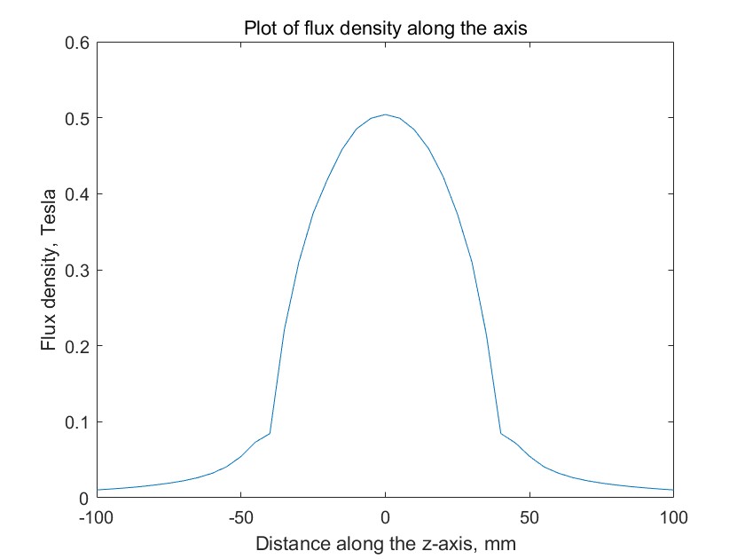
% If we were interested in the flux density at specific positions,
% we could inquire at specific points directly:
b0=mo_getb(0,0);
disp(sprintf('Flux density at the center of the bar is %f T',b0(2)));
b1=mo_getb(0,50);
disp(sprintf('Flux density at r=0,z=50 is %f T',b1(2)));
% Or we could, for example, plot the results along a line using
% Octave's built-in plotting routines:
zee=-100:5:100;
arr=zeros(1,length(zee));
bee=mo_getb(arr,zee);
plot(zee,bee(:,2))
xlabel('Distance along the z-axis, mm');
ylabel('Flux density, Tesla');
title('Plot of flux density along the axis');
% The program will report the terminal properties of the circuit:
% current, voltage, and flux linkage
vals = mo_getcircuitproperties('icoil');
% {i, v, \[Phi]} = MOGetCircuitProperties["icoil"]
% If we were interested in inductance, it could be obtained by
% dividing flux linkage by current
L = vals(3)/vals(1);
disp(sprintf('The self-inductance of the coil is %f mH',L*1000));
% When the analysis is completed, FEMM can be shut down.
closefemm
 |  |
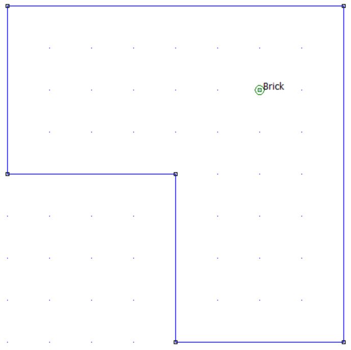
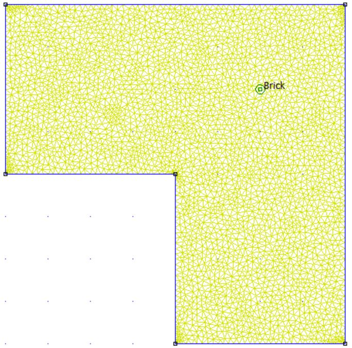
Auto-htutor (Flag=7)
openfemm
newdocument(2);

% define problem parameters
hi_probdef('meters','planar',1e-8,20,30);

% add in materials and boundary conditions
hi_addmaterial('Brick',0.7,0.7,0);
hi_addboundprop('Outer Boundary',2,0,0,300,5,0);
hi_addboundprop('Inner Boundary',2,0,0,800,10,0);

% draw the geometry
hi_drawpolygon([0,1; 0,2; 2,2; 2,0; 1,0; 1,1]);
hi_addblocklabel(1.5,1.5);

% apply the defined matrial to a block label
hi_selectlabel(1.5,1.5);
hi_setblockprop('Brick',0,0.05,0);
hi_clearselected
hi_zoomnatural

% apply the boundary conditions
hi_selectsegment(1,0.5);
hi_selectsegment(0.5,1);
hi_setsegmentprop('Inner Boundary',0,1,0,0,'<None>');
hi_clearselected
hi_selectsegment(2,0.5);
hi_selectsegment(0.5,2);
hi_setsegmentprop('Outer Boundary',0,1,0,0,'<None>');
hi_clearselected

% the file has to be saved before it can be analyzed.
hi_saveas('auto-htutor.feh');
hi_createmesh;
hi_analyze
% view the results
hi_loadsolution
% we desire to obtain the heat flux, just like in the
% tutorial example. first, define an integration contour
ho_seteditmode('contour');
ho_addcontour(0,1.5);
ho_addcontour(1.5,1.5);
ho_addcontour(1.5,0);
heatflux=ho_lineintegral(1);
disp(sprintf('The total heat flux is %f',4*heatflux(1)));

% if desired, the following line could be uncommented to
% shut down mirage:
closefemm
 |  |
The total heat flux is 59500.536492
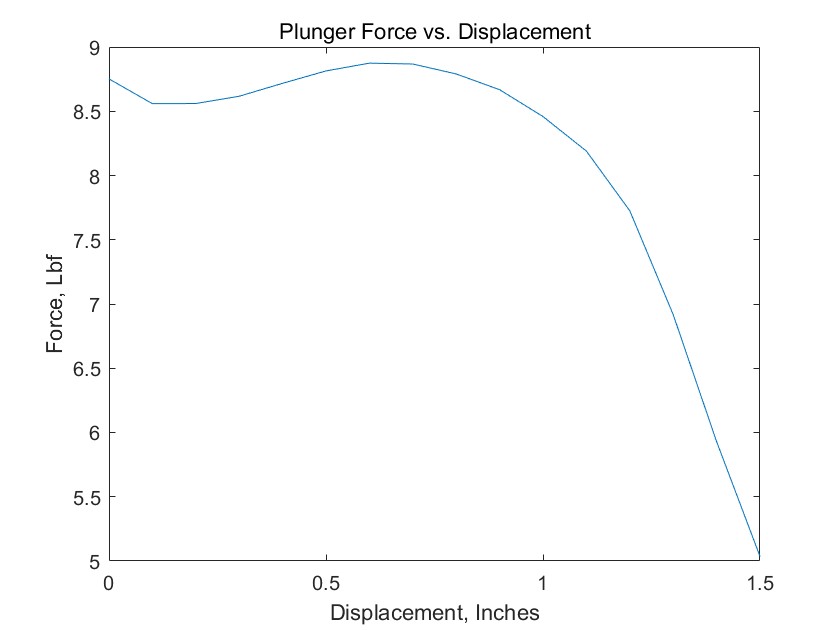
Roters1b: Simulation of a Tapered Plunger Magnet (Flag=8)
disp('Roters1b: Simulation of a Tapered Plunger Magnet');
disp('David Meeker');
disp('dmeeker@ieee.org');
disp('This geometry comes from Chap. IX, Figure 7 of Herbert Roters');
disp('classic book, Electromagnetic Devices.  The program moves');
disp('the plunger of the magnet over a stroke of 1.5in at 1/10in increments');
disp('solving for the field and evaluating the force on the plunger at');
disp('each position.  When all positions have been evaluated, the program');
disp('plots a curve of the finite element force predictions.');

openfemm

opendocument('roters1b.fem');
mi_saveas('temp.fem');
n=16;
stroke=1.5;
x=zeros(n,1);
f=zeros(n,1);

for k=1:n
  disp(sprintf('iteration %i of %i',k,n));
  mi_analyze;
  mi_loadsolution;
  mo_groupselectblock(1);
  x(k)=stroke*(k-1)/(n-1);
  f(k)=mo_blockintegral(19)/4.4481;
  mi_selectgroup(1);
  mi_movetranslate(0,-stroke/(n-1));
  mi_clearselected
end

plot(x,f)
xlabel('Displacement, Inches');
ylabel('Force, Lbf');
title('Plunger Force vs. Displacement');

closefemm
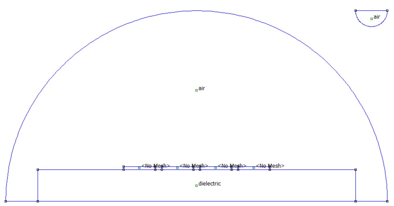
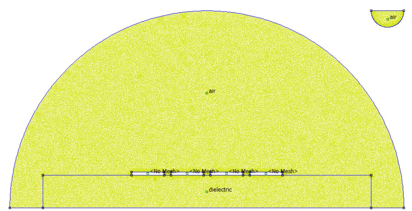
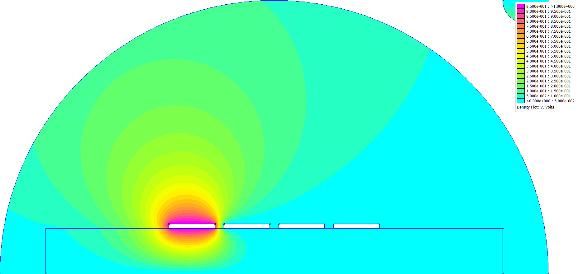
Strips (Flag=9)
disp('Electrostatics Example');
disp('David Meeker');
disp('dmeeker@ieee.org');
disp(' ');
disp('The objective of this program is to find the capacitance');
disp('matrix associated with a set of four microstrip lines on');
disp('top of a dielectric substrate. We will consider lines');
disp('that are 20 um wide and 2 um thick, separated by a 4 um');
disp('distance. The traces are laying centered atop of a 20 um');
disp('by 200 um slab with a relative permeability of 4. The');
disp('slab rests on an infinite ground plane. We will consider');
disp('a 1m depth in the into-the-page direction.');
disp(' ');
disp('This program sets up the problem and solves two different');
disp('cases with different voltages applied to the conductors');
disp('Becuase of symmetry, this yields enough information to');
disp('deduce the 4x4 capacitance matrix');
disp(' ');

% Start up and connect to FEMM
openfemm
% Create a new electrostatics problem
newdocument(1)

% Draw the geometry
ei_probdef('micrometers','planar',10^(-8),10^6,30);
ei_drawrectangle([2,0;22,2]);
ei_drawrectangle([2+24,0;22+24,2]);
ei_drawrectangle([-2,0;-22,2]);
ei_drawrectangle([-2-24,0;-22-24,2]);
ei_drawrectangle([-100,-20;100,0]);
ei_drawline([-120,-20;120,-20]);
ei_drawarc([120,-20;-120,-20],180,2.5);
ei_drawarc([100,100;120,100],180,2.5);
ei_drawline([100,100;120,100]);

% Create and assign a "periodic" boundary condition to
% model an unbounded problem via the Kelvin Transformation
ei_addboundprop('periodic',0,0,0,0,3);
ei_selectarcsegment(0,100);
ei_selectarcsegment(110,80);
ei_setarcsegmentprop(2.5,'periodic',0,0,'<none>');
ei_clearselected;

% Define the ground plane in both the geometry and the exterior region
ei_addboundprop('ground',0,0,0,0,0);
ei_selectsegment(0,-20);
ei_selectsegment(110,-20);
ei_selectsegment(-110,-20);
ei_selectsegment(110,100);
ei_setsegmentprop('ground',0,1,0,0,'<none>');
ei_clearselected;

% Add block labels for each strip and mark them with "No Mesh"
for k=0:3, ei_addblocklabel(-36+k*24,1); end
for k=0:3, ei_selectlabel(-36+k*24,1); end
ei_setblockprop('<No Mesh>',0,1,0);
ei_clearselected;
% Add and assign the block labels for the air and dielectric regions
ei_addmaterial('air',1,1,0);
ei_addmaterial('dielectric',4,4,0);
ei_addblocklabel(0,-10);
ei_addblocklabel(0,50);
ei_addblocklabel(110,95);
ei_selectlabel(0,-10);
ei_setblockprop('dielectric',0,1,0);
ei_clearselected;
ei_selectlabel(0,50);
ei_selectlabel(110,95);
ei_setblockprop('air',0,1,0);
ei_clearselected;

% Add a "Conductor Property" for each of the strips
ei_addconductorprop('v0',1,0,1);
ei_addconductorprop('v1',0,0,1);
ei_addconductorprop('v2',0,0,1);
ei_addconductorprop('v3',0,0,1);

% Assign the "v0" properties to all sides of the first strip
ei_selectsegment(-46,1);
ei_selectsegment(-26,1);
ei_selectsegment(-36,2);
ei_selectsegment(-36,0);
ei_setsegmentprop('<None>',0.25,0,0,0,'v0');
ei_clearselected

% Assign the "v1" properties to all sides of the second strip
ei_selectsegment(-46+24,1);
ei_selectsegment(-26+24,1);
ei_selectsegment(-36+24,2);
ei_selectsegment(-36+24,0);
ei_setsegmentprop('<None>',0.25,0,0,0,'v1');
ei_clearselected

% Assign the "v2" properties to all sides of the third strip
ei_selectsegment(-46+2*24,1);
ei_selectsegment(-26+2*24,1);
ei_selectsegment(-36+2*24,2);
ei_selectsegment(-36+2*24,0);
ei_setsegmentprop('<None>',0.25,0,0,0,'v2');
ei_clearselected

% Assign the "v3" properties to all sides of the fourth strip
ei_selectsegment(-46+3*24,1);
ei_selectsegment(-26+3*24,1);
ei_selectsegment(-36+3*24,2);
ei_selectsegment(-36+3*24,0);
ei_setsegmentprop('<None>',0.25,0,0,0,'v3');
ei_clearselected

 ei_zoomnatural;

% Save the geometry to disk so we can analyze it
ei_saveas('strips.fee');

% Analyze the problem
 ei_analyze

% Load the solution
ei_loadsolution
% Create a placeholder matrix which we will fill with capacitance values
c=zeros(4);
% Evaluate the first row of the capacitance matrix by looking at the charge on each strip
c(1,:)=[eo_getconductorproperties('v0')*[0;1],...
    eo_getconductorproperties('v1')*[0;1],...
    eo_getconductorproperties('v2')*[0;1],...
    eo_getconductorproperties('v3')*[0;1]];

% From symmetry, we can infer the fourth row of the matrix from the entries in the first row
 c(4,:)=c(1,:)*[0,0,0,1;0,0,1,0;0,1,0,0;1,0,0,0];

% Change the applied voltages so that the second conductor is set at 1 V and all others at 0V
ei_modifyconductorprop('v0',1,0);
ei_modifyconductorprop('v1',1,1);
ei_analyze;
eo_reload;

% Evaluate the second row of the capacitance matrix
c(2,:)=[eo_getconductorproperties('v0')*[0;1],...
    eo_getconductorproperties('v1')*[0;1],...
    eo_getconductorproperties('v2')*[0;1],...
    eo_getconductorproperties('v3')*[0;1]];

% And infer the third row from symmetry...
c(3,:)=c(2,:)*[0,0,0,1;0,0,1,0;0,1,0,0;1,0,0,0];

disp('The capacitance matrix is:');

% Now that we are done, shut down FEMM
closefemm
 |  |
参考文献
[1] OctaveFEMM Manual
本网站基于Hexo 3-Hexz主题生成。如需转载请标注来源,如有错误请批评指正,欢迎邮件至 392176462@qq.com