介绍
CoreLossCoeifficient用于拟合电工钢的BP曲线。
原理
Under sinusoidal flux conditions, core loss is computed in the frequency domain as follows:
$$
P_v=P_h+P_c+P_e=K_hf(B_m)^Y+K_c(fB_m)^2+K_e(fB_m)^{1.5}
$$
For a material with anisotropic core losses, the coefficients Kh, Kc, Ke, and Y have different values in different principal directions, that is, (Khx, Khy, Khz), (Kcx, Kcy, Kcz), (Kex, Key, Kez), and (Yx, Yy, Yz) in (x, y, z) directions, respectively.
where
Bm is the amplitude of the AC flux component,
f is the frequency,
Kh is the hysteresis core loss coefficient,
Kc is the eddy-current core loss coefficient, and
Ke is the excess core loss coefficient.
Y is the power of Bm for hysteresis core loss.
类结构
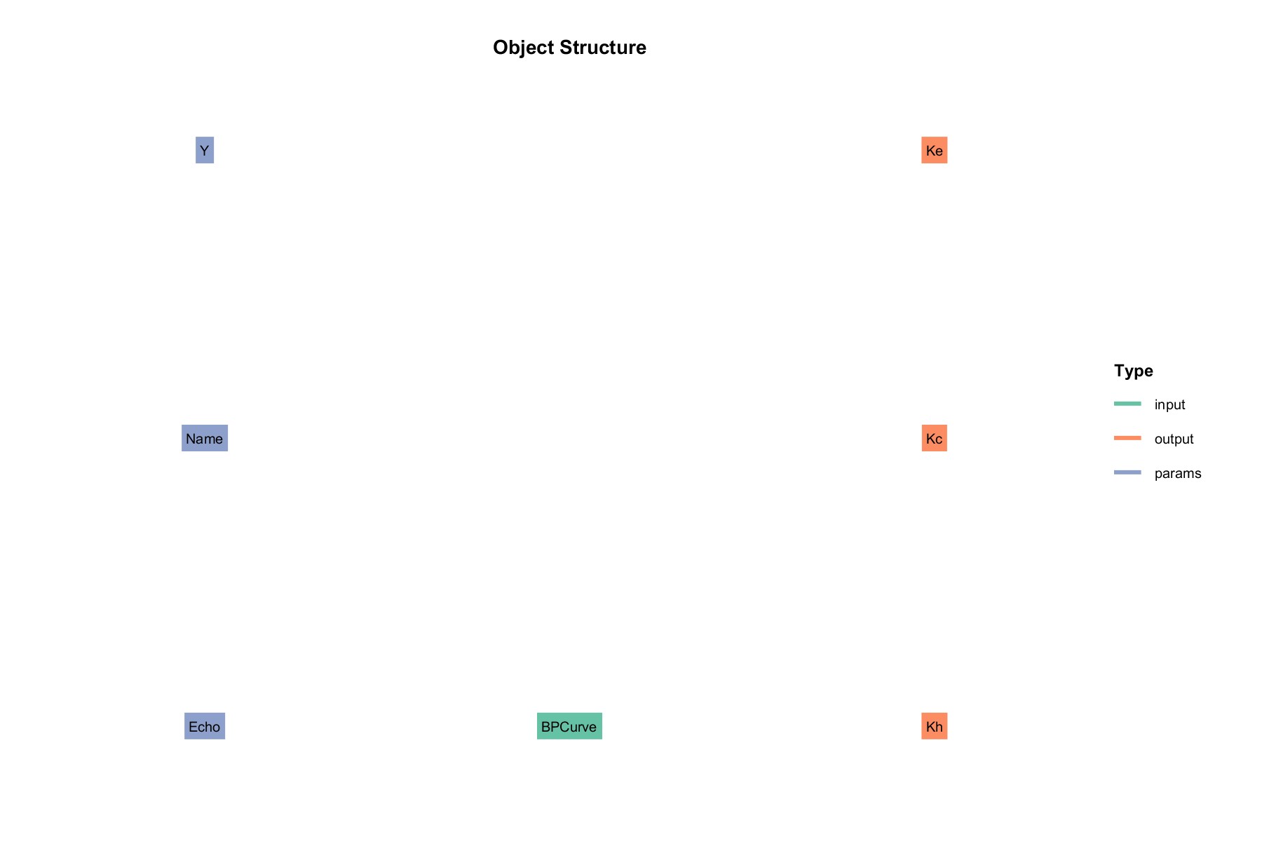
输入 input:
- BPCurve : BP曲线测试值
参数 params:
- Y :参数
- Name : 名称
输出 output :
- Kh : 磁滞损耗参数
- Kc : 涡流损耗参数
- Ke : 其他损耗参数
案例
sz = [1 12];
varTypes = {'cell','cell','cell','cell','cell','cell','cell','cell','cell','cell','cell','cell'};
varNames = {'50','60','100','200','400','600','700','800','1000','2000','5000','10000'};
Curve = table('Size',sz,'VariableTypes',varTypes,'VariableNames',varNames);
Curve=ReadData(Curve);
inputStruct1.BPCurve=Curve;
paramsStruct1=struct();
Mat= method.CoreLossCoeifficient(paramsStruct1, inputStruct1);
Mat= Mat.solve();
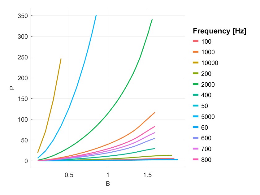
PlotinputCurve(Mat);
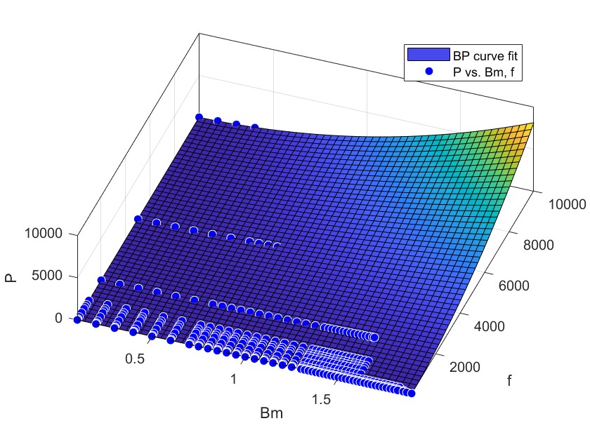
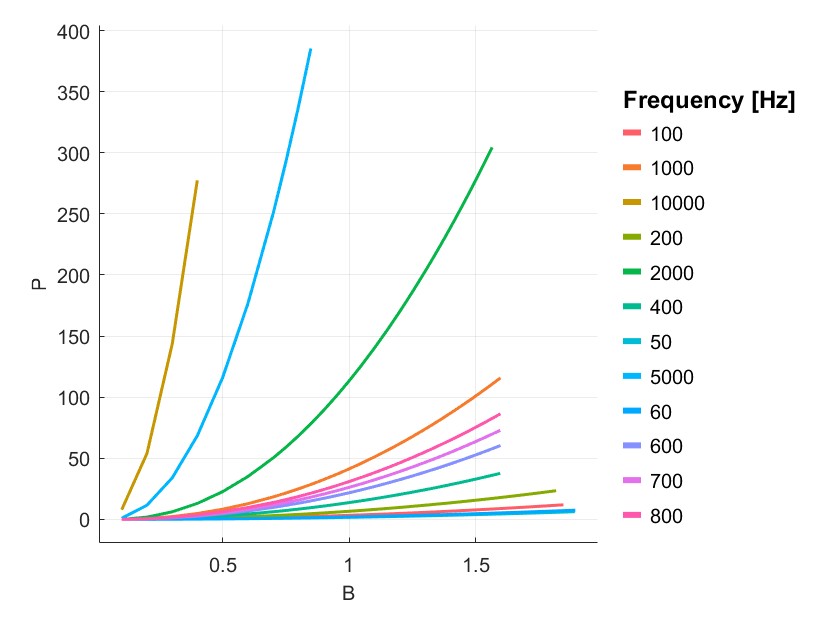
PlotFitCurve(Mat);
 |  |
参考文献
本网站基于Hexo 3-Hexz主题生成。如需转载请标注来源,如有错误请批评指正,欢迎邮件至 392176462@qq.com